Quantitative Genetics, Coancestry and Status Number

Coancestry ( , f) between pair of individuals is the probability that genes, taken at random from each of the concerned individuals, are identical by descent (=coefficient of coancestry). Kinship is equivalent. Wright’s coefficient of relationship is less practical.

The chance that both homologous genes in the same zygote are identical by descent is called inbreeding (F) (or coefficient of inbreeding).

If two individuals mate, their coancestry becomes the inbreeding of their offspring.

Founder population is the starting point of calculations. If all inbreeding and coancestry of the founder population is known, inbreeding and coancestry can be calculated from a pedigree. It is usually practical and convenient to set inbreeding and coancestry to zero in the "wild forest" (or source population) and see the founders (plus trees) as a sample from the wild forest.

Inbreeding and coancestry are relative to some real or imaginary "base" or "reference" or "source" population. Most conveniently this is the founder population or the wild forest.

Self-coancestry: An individual's coancestry with itself is 0.5(1+F).

This can be realised e.g. by considering that coancestry in the previous generation becomes inbreeding in next, and then consider selfing.

Gene pool means all genes in a population. It is convenient to consider genes at one locus. The gene pool is independent on how (or if) a population is organised in zygotes.

Genes in a gene pool

A population with N zygotes has 2N genes in the gene pool

Each gene has the frequency 1/2N

Arrows = sampling with replacement (or infinite copies of each gene)

Probability to sample the same gene twice is 1/2N

Probability that different genes will be sampled is (1-0.5/N).

Genes can be IBD (identical by descent). The probability is the coancestry.

Individuals versus Gene Pool

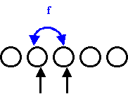
The gene pool is structured in individuals

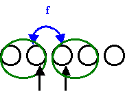
The probability that the genes in two specific individuals are IBD is the coancestry between these two individuals.

The probability that the different genes in the same zygote are IBD is the coefficient of inbreeding.

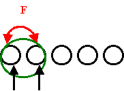
For self-coancestry the genes need not to be different. If they are different f=F, if the same f=1, average f=(1+F)/2.

Three different mechanisms genes sampled in the current population may be IBD:

1. The same gene sampled twice (drift);

2. The genes are homologous genes from the same individual (inbreeding),

3. The genes originate from different individuals (relatedness).

The values of the pair-wise coancestries of individuals can be arranged in a coancestry matrix

Ind	1	2	3
1	0.5	0.25	0
2	0.25	0.5	0
3	0	0	1

We denote a certain value by f_2,1=0.25

Note that a covariance matrix is symmetric, thus f_2,1= f_1,2

The values along the diagonal (self-coancestries) appear only once.

Coefficient of relationship are often arranged in such a matrix, (numerator matrix), in absence of inbreeding these values are double as large.

Coancestries are probabilities, thus f between 0 and 1.

Some examples of coancestries

Relative	Coancestry
Unrelated	0
Half sibs	0.125
Full sibs	0.25
Parent-offspring	0.25
Cousin	0.0625
Itself (self-coancestry)	0.5

Group coancestry

Let's put all homologous genes in a big pool and select two (at random with replacement). The probability that two are IBD we define as group coancestry. (, this term was introduced by Cockerham 1967).

To get overall probability; average over all individual probabilities, f.

Group coancestry equals the average of all N² coancestry values among all combinations of the N individuals in a population (or the average of all 4N² combinations of individual genes). We could as well define group coancestry as this average, the advantage of the probabilistic definition appears in more complex situations.

Average coancestry

Let’s form the average of the coancestry matrix for three individuals

Ind	1	2	3
1	0.5	0.25	0
2	0.25	0.5	0
3	0	0	1

Sum of the 9 values in matrix= 2.5; Average = group coancestry = 2.5/9 = 0.278

Note that self-coancestries appear once, while other coancestries appear twice (reciprocals).

Group coancestry is here this average, but still a wider concept.

If all individuals in a population are of the same type, it is enough to calculate the N coancestries for a single individual.

Self-coancestry is the group coancestry for a population with a single member.

All members in a full sib family have equal coancestries to all other individuals. Thus it is enough to construct the coancestry matrix for full sib families (and make some thinking).

Group coancestry depends on relatedness, not how uniting gametes are arranged. A brother is equally related to his brother as to his sister, in spite of that his gametes are able to unite only with those of his sister.

Cross-coancestry, Inbreeding and Group Coancestry relations

The term cross-coancestry is used here for the average of all coancestries among individuals excepting self-coancestry. "Average group cross-coancestry" seems unneeded complicated. However, "Coancestry" in the meaning "average cross-coancestry" invites to misunderstandings.

If inbreeding and coancestry are known in a population, group coancestry can be calculated.

Using these relationships, formulas for group coancestry and average cross-coancestry as a function of parameters for the current population can be derived

There = group coancestry; N = individuals;

= cross-coancestry; =average inbreeding

Linking generations

Group coancestry changes at generation shifts are possible to calculate retrospectively from a known pedigree linking to the founders.

Future group coancestry can be calculated with knowledge about future pedigrees.

For other cases predictions may be made, but they are often far from trivial.

Note also that there may be doubt if assumptions are realistic (neutral selection, many genes with infinitesimal action etc.)
The link between the generations is the gametes.

The gene pool of the offspring is identical to the gene pool of the successful gametes of the parents.

Consider a pair of genes, which may equivalently be regarded as in offspring zygotes or in parental successful gametes!

A pair of genes may be IBD as they are copies of the same gene in the parent population. This may happen if a parent get more than one offspring.

A pair of genes may originate from homogenous genes of the same parental zygote in the parental generation, if that was inbred the considered genes may be IBD.

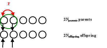
Two gametes from the same parent has coancestry (1+F_parent)/2. Sibs who share that parent get coancestry (1+F_parent)/8 (there may be a contribution from the other parent also).

If the considered gene pair originates from different parents, the coancestry will be f_parent.

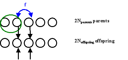
IBD may occur by the following mechanisms:

1. The same gene in the current generation is sampled twice,

2. The genes are copies of the same gene in the parental generation,

3. The genes origin from homologous genes in the same inbred parent,

4. The genes come from different, but related, parents.

Group coancestry and gene diversity

Group coancestry is the probability that two genes in a population are IBD.

Diversity means that things are different, gene diversity means that genes are different.

Evidently 1-group coancestry is the probability that the genes are non-identical, thus diverse.

is a measure of gene diversity and group coancestry is a measure of Gene Diversity lost compared to the reference population.

This way of thinking assumes all genes in individuals in the reference populations are unique.

Group coancestry based measures are relative to a reference population.

GD is expected average heterozygosity.

For forest tree breeding the wild forest often constitutes a good reference. The gene diversity of the wild forest is 1, and the group coancestry will give the percentage of gene diversity lost.

If we monitor group coancestry in our tree improvement operations, we can say how much gene diversity has been lost compared to the wild forest.

An algorithm for calculation of coancestry and group coancestry

(the example can be found in Lindgren et al 1997).

Pedigree for a population used as example

Points (.) for founders. Parents always defined as individuals before as parents.

Ind	Parent A	Parent B
1	.	.
2	.	.
3	.	.
4	.	.
5	1	1
6	2	3
7	2	3
8	3	4
9	.	.
10	5	6
11	7	8
12	8	9
13	9	.

The pedigree in the Table can be visualised in the following way:

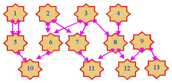
1, 2, 3, 4, 9 and an unknown parent to 13 can be considered as "founders"

The group coancestry for a group consisting of 10, 11, 12 and 13 will be derived in the following

Calculation of the coancestry matrix.

The pedigree used is shown above

Fill the matrix (thus the coancestry of all pair of individuals) using the pedigree information.

This can be done step by step using the already filled in part of the matrix.

Fill a row

Start with the diagonal element

Proceed left to the end

As the matrix is symmetrical the column values can be filled in from the row

Start with next diagonal
The matrix below has been filled to element (6,6). Individual 6 which has parents 2 and 3, individual 8 parents 3 and 4 it is demonstrated how elements (6,6) and (6,8) are filled.

Ind	1	2	3	4	5	6	7	8	9	10	11	12	13
1	0.5	0	0	0	0.5	0	0	0	0	0.25	0	0	0
2	0	0.5	0	0	0	0.25	0.25	0	0	0.125	0.125	0	0
3	0	0	0.5	0	0	0.25	0.25	0.25	0	0.125	0.25	0.125	0
4	0	0	0	0.5	0	0	0	0.25	0	0	0.125	0.125	0
5	0.5	0	0	0	0.75	0	0	0	0	0.375	0	0	0
6	0	0.25	0.25	0	0	0.5	0.25	0.125
7	0	0.25	0.25	0	0
8	0	0	0.25	0.25	0
9	0	0	0	0	0
10	0.25	0.125	0.125	0	0.375
11	0	0.125	0.25	0.125	0
12	0	0	0.125	0.125	0
13	0	0	0	0	0

The diagonal: average of 0.5 and coancestry for parents 2 and 3

(6,6)=0.5+(3,2)=0.5+0

The off diagonal: average of coancestry with 6 and the parents to 8 (3 and 4)

(6,8)=0.5[(6,3)+(6,4)]=0.5[0.25+0]=0.125

(the average of the parents to 7’s coancestry with 6)

The complete coancestry matrix. Group coancestry for 10-13

Ind	1	2	3	4	5	6	7	8	9	10	11	12	13
1	0.5	0	0	0	0.5	0	0	0	0	0.25	0	0	0
2	0	0.5	0	0	0	0.25	0.25	0	0	0.125	0.125	0	0
3	0	0	0.5	0	0	0.25	0.25	0.25	0	0.125	0.25	0.125	0
4	0	0	0	0.5	0	0	0	0.25	0	0	0.125	0.125	0
5	0.5	0	0	0	0.75	0	0	0	0	0.375	0	0	0
6	0	0.25	0.25	0	0	0.5	0.25	0.125	0	0.25	0.188	0.063	0
7	0	0.25	0.25	0	0	0.25	0.5	0.125	0	0.125	0.313	0.063	0
8	0	0	0.25	0.25	0	0.125	0.125	0.5	0	0.063	0.313	0.25	0
9	0	0	0	0	0	0	0	0	0.5	0	0	0.25	0.25
10	0.25	0.125	0.125	0	0.375	0.25	0.125	0.063	0	0.5	0.094	0.031	0
11	0	0.125	0.25	0.125	0	0.188	0.313	0.313	0	0.094	0.563	0.156	0
12	0	0	0.125	0.125	0	0.063	0.063	0.25	0.25	0.031	0.156	0.5	0.125
13	0	0	0	0	0	0	0	0	0.25	0	0	0.125	0.5

The red population get the red coancestry values, the group coancestry for the population 10-13 is the average of the red values (= 2.875/16=0.1797).

Status number
Status number is the half the inverse of group coancestry

Or, equivalently
Status number is half the inverse of the probability that two genes drawn at random are IBD.

An attractive property of the status number is that it is the same as the census number for a population of unrelated, non-inbred individuals. The status number says that the probability to draw two genes IBD is the same as if it were so many unrelated non-inbred individuals contributing to the gene pool. Therefore we can call it an effective number.

Status number is an intuitively appealing way of presenting group coancestry, as it connects to the familiar concept of number (population size).

The ratio of the status number and the census number will be useful, thus N_r=N_s/N. I call this the relative status number.

The drop of Gene Diversity

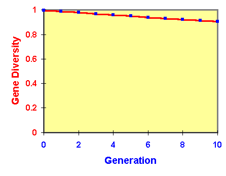
This is to exemplify what may happen to Gene Diversity during breeding (from Lindgren et al 1997).

Data from a simulated breeding program. POPSIM simulation; Breeding Populatin=100; four controlled matings made for each member of the breeding population, the family size was 40, the next generation was recruited from the previous by phenotypic selection (selecting the best 100 among the offspring considering only the phenotype), the initial heritability was 0.2.

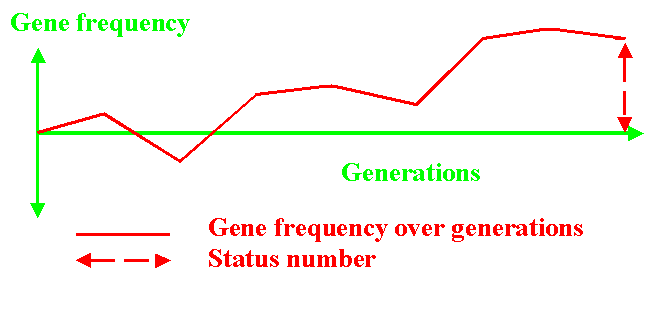
Status number and group coancestry measure gene dispersion! Cockerham (1969) concluded that the variance of the gene frequency (that’s the mean of the occurrence of a gene) is

this can equivalently be expressed

This is the binomial expression of the variance for the gene frequency in a population with N_s non-inbred non-related members!

Status number is the size of unrelated non inbred trees sampled from the reference population, which have the same drift as the accumulated drift of the population under study (compared to the reference population).

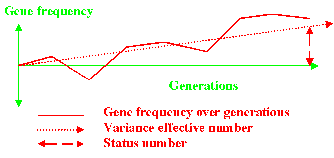
Status number, group coancestry and variance effective number

The concepts may (in an over-simplified world) be linked

, when N_V is large

where N_S = status number N_V variance effective number and t generations

Can also be expressed

However, the initial founders matters, so the formulas are more relevant for the development over generations that the absolute values.

Group coancestry and Wright's F-statistics

What is called F_IS is the difference between inbreeding and cross-coancestry. If Hardy-Weinberg balance they are equal (the same chance of IBD if the genes are in the same as in different individuals).

I have developed the relations with Q as follows

Forest tree breeding and status number

The status number concept is more useful to forest tree breeders than other breeders or geneticists. Forest tree breeders

are still very close to the founders

thus close to the "wild forest"

deal with few generations

change strategy between generations

structure population in sublines

"own" and control the breeding population